Final Post: Gamex and Faces in Baroque Paintings

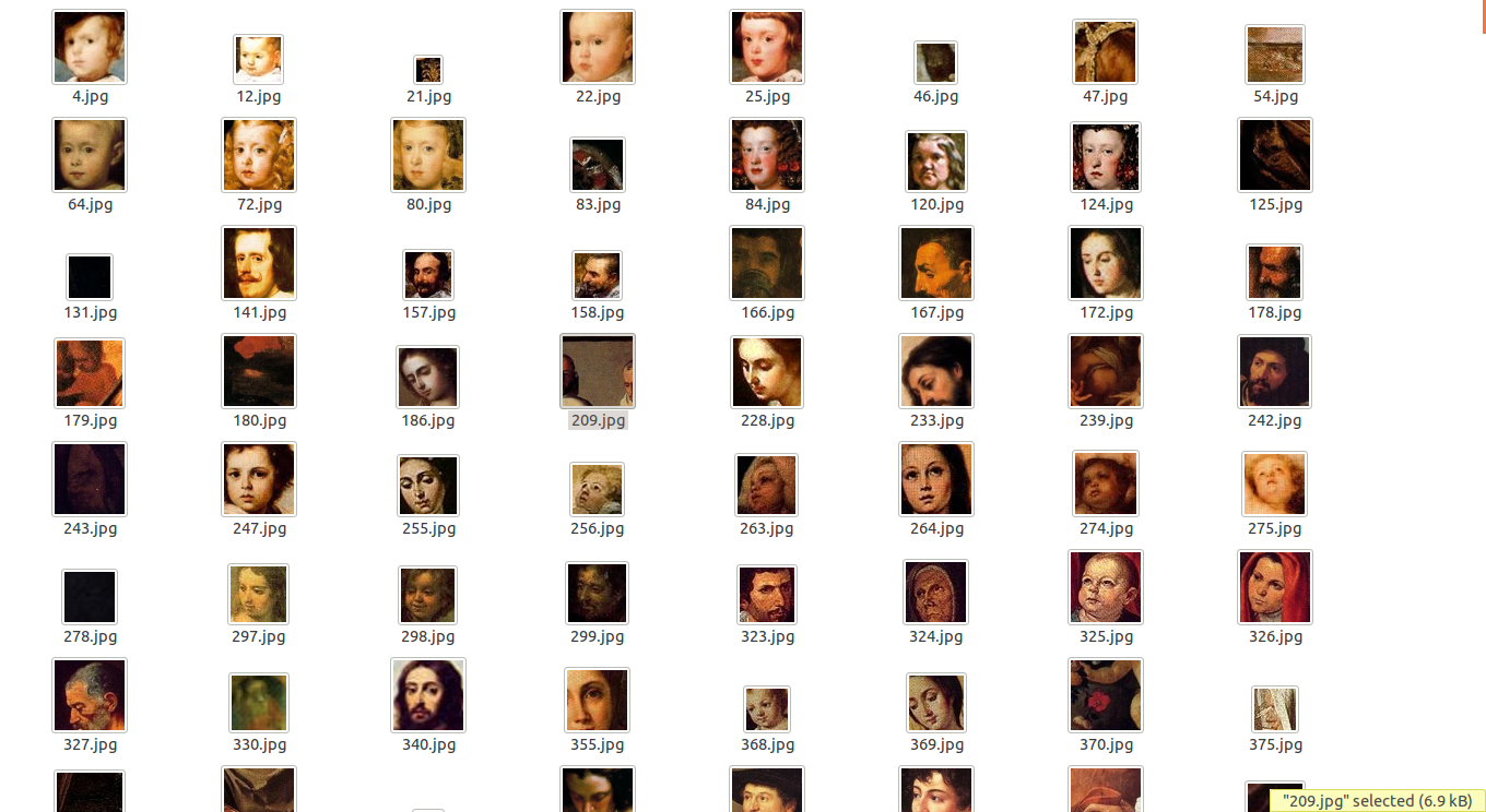
Face recognition algorithms (used in digital cameras) allowed us to detect faces in paintings. This has gave us the possibility of having a collection of faces of a particular epoch (in this case, the baroque). However, the results of the algorithms are not perfect when applied in paintings instead of pictures. Gamexgives the chance to clean this collection. This is very important since these paintings are the only historical visual inheritance we have from the period. A period that started after the meet of two worlds.

1. Description

Gamex was born from the merging of different ideas we had at the very beginning of the Interactive Exhibit Design course. It basically combines motion detection, face recognition and games to produce an interactive exhibit of Baroque paintings. The user is going to interact with the game by touching, or more properly poking, faces, eyes, ears, noses, mouths and throats of the characters of the painting. We will be scoring him if there is or there is not a face already recognized on those points. Previously, the database has a repository with all the information the faces recognition algorithms have detected. With this idea, we will be able to clean mistakes that the automatic face recognition has introduced.

2. The Architecture

A Tentative Architecture for Gamex explains the general architecture in more detail. Basically we have four physical components:

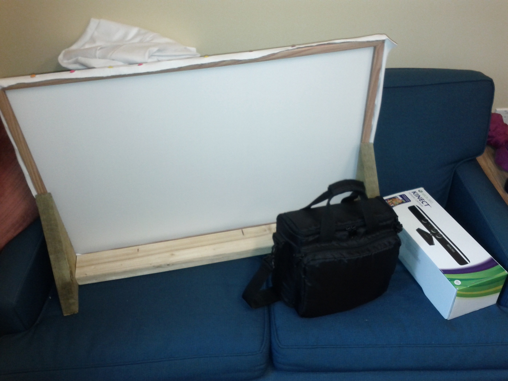
A screen. Built with a wood frame and elastic-stretch fabric where the images are going to be projected from the back and where the user is going to interact poking them.
The projector. Just to project the image from the back to the screen (rear screen projetion).
Microsoft Kinect. It is going to capture the deformations on the fabric and send them to the computer.
Computer. Captures the deformations send by the Kinect device and translates them to touch events (similar to mouse clicks). These events are used in a game to mark on different parts of the face of people from baroque paintings. All the information is stored in a database and we are going to use it to refine a previously calculated set of faces obtained through face recognition algorithms.

3. The Technology

There were several important pieces of technology that were involved in this project.

Face Recognition

Recent technologies offers us the possibility of recognizing objects in digital images. In this case, we were interested in recognizing faces. To achieve that, we used the libraries OpenCV and SimpleCV. The second one just allowed us to use OpenCV with Python, the glue of our project. There are several posts in which we explain a bit more the details of this technology and how we used.

Multi Touch Screen

One of the biggest part of our work involved working with multi-touch screens. Probably because it is still a very new technology where things haven’t set down that much we have several problems but fortunately we managed to solved them all. The idea is to have a rear screen projection using the Microsoft Kinect. Initially though for video-game system Microsoft Xbox 360, there is a lot of people creating hacks (such as Simple Kinect Touch) to take advantage of the abilities of this artifact to capture deepness. Using two infrared lights and arithmetic, this device is able to capture the distance from the Kinect to the objects in front of it. It basically returns an image, in which each pixel is the deepness of the object to the Kinect. All sorts of magic tricks could be performed, from recognizing gestures of faces to deformations in a piece of sheet. This last idea is the hearth of our project. Again, some of the posts explaining how and how do not use this technology.

Games

Last but not least, Kivy. Kivy is an open source framework for the development of applications that make use of innovative user interfaces, such as multi-touch applications. So, it fits to our purposes. As programmers, we have developed interfaces in many different types of platforms, such as Java, Microsoft Visual, Python, C++ and HTML. We discovered Kivy being very different from anything we knew before. After struggling for two or three weeks we came with our interface. The real thing about Kivy is that they use a very different approach which, apart from having their own language, the developers claim to be very efficient. At the very end, we started to liked and to be fair it has just one year out there so it will probably improve a lot. Finally, it has the advantage that it is straightforward to have a version for Android and iOS devices.

4. Learning

There has been a lot of personal learning in this project. We never used before the three main technologies used for this project. Also we included a relatively new NoSQL database system called MongoDB. So that makes four different technologies. However, Javier and me agree that one of the most difficult part was building up the frame. We tried several approaches: from using my loft bed as a frame to a monster big frame (with massive pieces of wood carried from downtown to the university in my bike) that the psyco duck would bring down with the movement of the wings.

It is also interesting how ideas changes over the time, some of them we probably forgot. Others, we tried and didn’t work as expected. Most of them changed a little bit but the spirit of our initial concept is in our project. I guess creative process is a long way between a driven idea and the hacks to get to it.

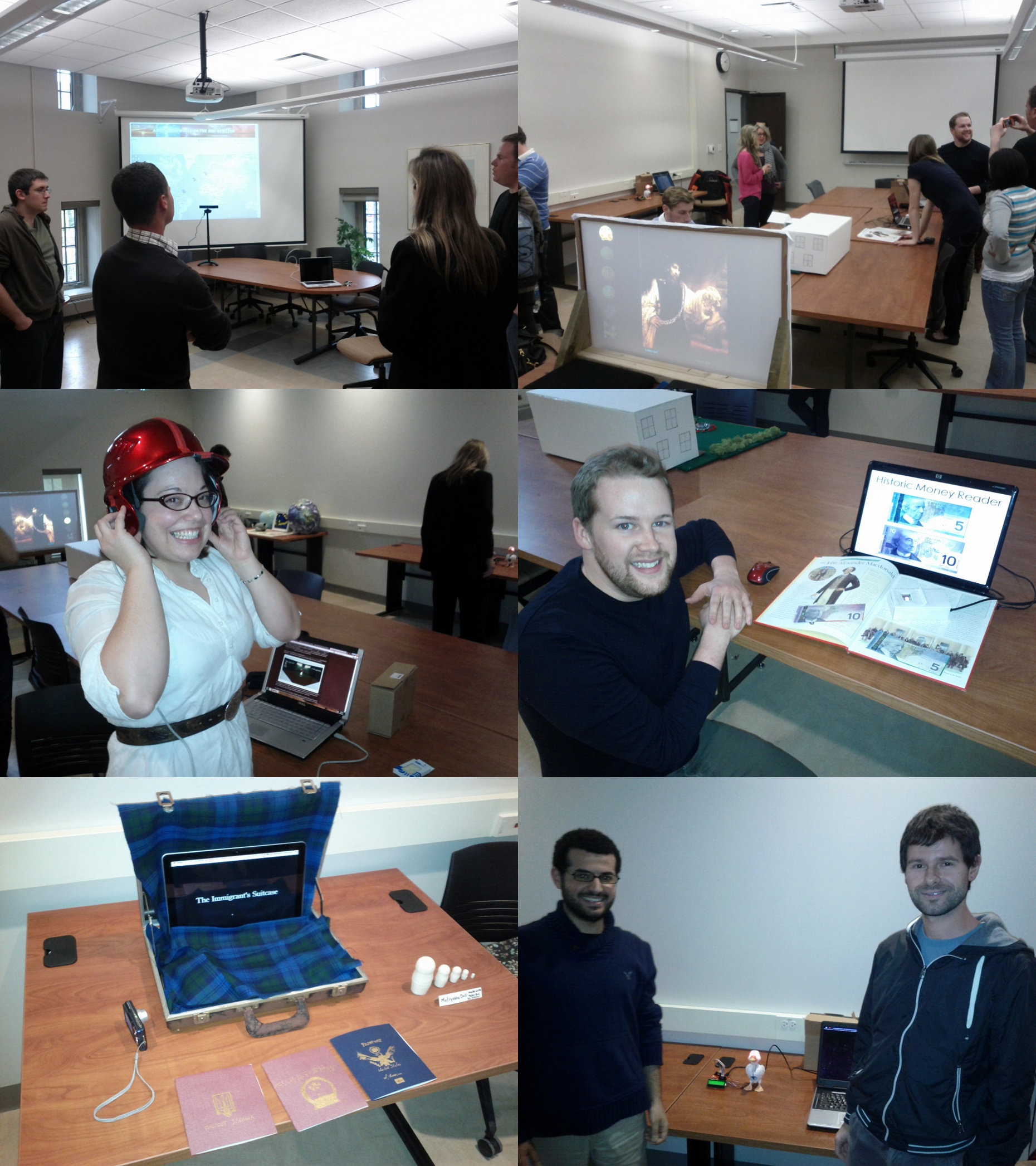
5. The Exhibition

Technology fails on the big day and the day of the presentation we couldn’t get our video but there is the ThatCamp coming soon. A new opportunity to see users in action. So the video of the final result, although not puclib yet, is attached here. It will come more soon!

[youtube BVYq_cBf8z4]

6. Future Work

This has been a long post but there is still a few more things to say. And probably much more in the future. We liked the idea so much that we are continuing working on this and we liked to mention some ideas that need to be polished and some pending work:

Score of the game. We want to build a better system for scores. Our main problem is that the data that we have to score is incomplete and imperfect (who has always the right answers anyway). We want to give a fair solution to this. Our idea is to work with fuzzy logic to lessen the damage in case the computer is not right.
Graphics. We need to improve our icons. We consider some of them very cheesy and needs to be refined. Also, we would like to adapt the size of the icon to the size of the face the computer already recognized, so the image would be adjusted almost perfectly.
Sounds. A nice improvement but also a lot of work to have a good collection of midi or MP3 files if we don’t find any publicly available.
Mobile versions. Since Kivy offers this possibility, it would be silly not to take advantage of this. At the end, we know addictive games are the key to entertain people on buses. This will convert the application in a real crowd sourcing project. Even if this implies to build a better system for storing the information fllowing the REST principles with OAuth and API keys.
Cleaning the collection. Finally, after having enough data it would be the right time to collect the faces and have the first repository of “The Baroque Face”. This will give us an spectrum of how does the people of the XVI to XVIII looked like. Exciting, ¿isn’t it?
Visualizations. Also we will be able to do some interesting visualizations, like heat maps where the people did touch for being a mouth, or an ear, or a head.

6. Conclusions

In conclusion we can say that the experience has been awesome. Even better than that was to see the really high level of our classmates’ projects. In the honour of the truth, we must say that we have a background in Computer Science and we played somehow with a little bit more of adventage. Anyway, it was an amazing experience the presentation of all the projects. We really liked the course and we recommend to future students. Let’s see what future has prepared for Gamex!

This post was written and edit togetter with my classmate Javier. So you also can find the post on his blog.

One of the most important ideas in object recognition, particularly faces recognition, became with the work of Viola and Jones [1]. This work is based in the algorithm of Adaboost [2]. The idea is use very simple features of the faces that can be calculated very fast. Then select the best ones testing against a previously set of faces. In general, a feature is any value we can extract from a digital image. For example, a simple value of a pixel could be a feature. It is also possible to use more sophisticated stuff like histograms of colors or edges. In the case of Viola and Jones they use a very simple way of play with pixels. Just as an example, a feature could be the substraction of the area (sum of pixels) of one region of the image to another region of the image.

So, as part of the course Interactive Exhibit Design we decided to use this. Then I processed a lot of old baroque paintings and extract the faces. Even though the results are not perfect, I obtained decent results. I have a whole folder of faces and these are two sections of it. the first is a good section of the folder and the second a not-so-good section. I hope to do something interesting with all of this.

[1] Rapid object detection using a boosted cascade of simple features

[2] A decision-theoretic generalization of on-line learning and an application to boosting

This post follow the same idea as Lots of features from color histograms on a directory of images but using Edge orientation histograms in global and local features.

Basically I wanted to construct a collection of different edge orientation histograms for a collection of images that were saved in a directory. The histograms were calculated in different regions so I could get a lot of features. The images were numerated so the name of the file coincides with a number. The first thing I noticed was that I shouldn't use the code of Edge orientation histograms in global and local features directly because it was very inefficient. There is no need of calculating the gradients each time. It is better to do it just once and then extract the histogram from regions of this initial process. For this reason I divided that function in two functions: extract_edges and hist_edges. Here are both codes:

# parameters
# - the image
function [data] = extract_edges(im)

% define the filters for the 5 types of edges
f2 = zeros(3,3,5);
f2(:,:,1) = [1 2 1;0 0 0;-1 -2 -1];
f2(:,:,2) = [-1 0 1;-2 0 2;-1 0 1];
f2(:,:,3) = [2 2 -1;2 -1 -1; -1 -1 -1];
f2(:,:,4) = [-1 2 2; -1 -1 2; -1 -1 -1];
f2(:,:,5) = [-1 0 1;0 0 0;1 0 -1];

% the size of the image
ys = size(im,1);
xs = size(im,2);

# The image has to be in gray scale (intensities)
if (isrgb(im))
    im = rgb2gray(im);
endif

# Build a new matrix of the same size of the image
# and 5 dimensions to save the gradients
im2 = zeros(ys,xs,5);

# iterate over the posible directions
for i = 1:5
    # apply the sobel mask
    im2(:,:,i) = filter2(f2(:,:,i), im);
end

# calculate the max sobel gradient
[mmax, maxp] = max(im2,[],3);
# save just the index (type) of the orientation
# and ignore the value of the gradient
im2 = maxp;

# detect the edges using the default Octave parameters
ime = edge(im, 'canny');

# multiply against the types of orientations detected
# by the Sobel masks
data = im2.*ime;

function [data] = histo_edges(im, edges, r)

% size of the image
ys = size(im,1);
xs = size(im,2);
size = round(ys/r) * round(xs/r);

# produce a structur to save all the bins of the
# histogram of each region
eoh = zeros(r,r,6);
# for each region
for j = 1:r
    for i = 1:r
        # extract the subimage
        clip = edges(round((j-1)*ys/r+1):round(j*ys/r),round((i-1)*xs/r+1):round(i*xs/r));
        # calculate the histogram for the region
        eoh(j,i,:) = (hist(makelinear(clip), 0:5)*100)/numel(clip);
    end
end

# take out the zeros
eoh = eoh(:,:,2:6);

# represent all the histograms on one vector
data = zeros(1,numel(eoh));
data(:) = eoh(:);

Now, with this two functions and following the idea of Lots of features from color histograms on a directory of images, it is possible to generate the features in just one vector for each of the images:

function [t_set] = extract_eohs(dir, samples, filename)

fibs = [1,2,3,5,8,13];
total = 0;
ranges = [6, 2];
for fib = 1:size(fibs)(2)
    ranges(fib,1) = total + 1;
    total += 5*fibs(fib)*fibs(fib);
    ranges(fib,2) = total;
endfor

histo = zeros(samples, total);

for ind = 1:samples
    im = imread(strcat(dir, int2str(ind)));
    edges = extract_edges(im);
    for fib = 1:size(fibs)(2)
        histo(ind,ranges(fib,1):ranges(fib,2)) = histo_edges(im, edges, fibs(fib));
    endfor
endfor
save("-text", filename, "histo");
save("-text", "ranges.dat", "ranges");

t_set = ranges;

In my last course of computer vision and learning, I was working on a project to recognize between two styles of paintings. I decided to use the Adaboost algorithm [1]. I am going to describe the steps and code to make the algorithm run.

Step 0. The binary classification

This is not a step, but you have to be clear that this algorithm is just for classifying two classes. For example, ones from zeros, faces from non-faces or, in my case, baroque from renaissance paintings.

Step 1. Prepare the files.

There are several ways of introducing the samples to the algorithm. I found that the easiest way was using simple csv files. Also, you DO NOT have to worry about dividing the samples in training or testing. Just put all in the same files, OpenCV is going to divide the set picking the training/testings samples automatically. Then it is a good idea to put all the samples of the first class at the beginning and the second class at the end.

The format is very simple. The first column is going to be the category (however you can specify the exact column if your file does not follow this format). The rest of the columns are going to be the features of your problem. For example, I could have used three features. Each of them represent the average of red, blue and green per pixel in the image. So my csv file should look like this. Note that in the first column I am using a character. I recommend to do that so OpenCV is going to recognize that is a category (again you could specify that this a category an not a number).

B,124.34,45.4,12.4
B,64.14,45.23,3.23
B,42.32,125.41,23.8
R,224.4,35.34,163.87
R,14.55,12.423,89.67
...

NOTE: For a very strange reason the OpenCV implementation does not work with less than 11 samples. So this file should have at leas 11 rows. Just put some more to be sure and because you will need to specify a testing set as well.

Step 2. Opening the file

Let's suppose that the file is called "samples.csv" This would be the code:

 //1. Declare a structure to keep the data
CvMLData cvml;
//2. Read the file
cvml.read_csv("samples.csv");
//3. Indicate which column is the response
cvml.set_response_idx(0);

Step 3. Splitting the samples

Let's suppose that our file has 100 rows. This code would select 40 for the training.

 //1. Select 40 for the training
CvTrainTestSplit cvtts(40, true);
//2. Assign the division to the data
cvml.set_train_test_split(&cvtts);

Step 4. The training process

Let's suppose that I got 1000 features (columns in the csv after the response) and that I want to train the algorithm with just 100 (the second parameter in the next code)

 //1. Declare the classifier
CvBoost boost;
//2. Train it with 100 features
boost.train(&cvml, CvBoostParams(CvBoost::REAL, 100, 0, 1, false, 0), false);

The description of each of the arguments can be find here.

Step 5. Calculating the testing and training error

The error corresponds to the misclassified samples. Then, there could be two possible errors: the training and the testing.

 // 1. Declare a couple of vectors to save the predictions of each sample
std::vector train_responses, test_responses;
// 2. Calculate the training error
float fl1 = boost.calc_error(&cvml,CV_TRAIN_ERROR,&train_responses);
// 3. Calculate the test error
float fl2 = boost.calc_error(&cvml,CV_TEST_ERROR,&test_responses);

Note that the responses for each samples are saved in the train_responses and test_responses vectors. This is very useful to calculate confusion matrix (false positives, false negatives, true positives and false negatives and roc curves. I ll be posting how to build them with R.

Step 6. Save your classifier!!

You probably wouldn't mind at the beginning when it takes a few seconds to train something but you definitely don't want to lost it after a couple of hours or days that you waited for the results:

 // Save the trained classifier
boost.save("./trained_boost.xml", "boost");

Step 7. Compiling the whole code

The whole code is pasted at the end. To compile it, use this

g++ -ggdb `pkg-config --cflags opencv` -o `basename main` main.cpp `pkg-config --libs opencv`;

Here is the file with my code.

[1] http://citeseerx.ist.psu.edu/viewdoc/summary?doi=10.1.1.56.9855

#main.cpp
#include <cstdlib>
#include "opencv/cv.h"
#include "opencv/ml.h"
#include <vector>

using namespace std;
using namespace cv;
int main(int argc, char** argv) {

/* STEP 2. Opening the file */
//1. Declare a structure to keep the data
CvMLData cvml;
//2. Read the file
cvml.read_csv("samples.csv");
//3. Indicate which column is the response
cvml.set_response_idx(0);

/* STEP 3. Splitting the samples */
//1. Select 40 for the training
CvTrainTestSplit cvtts(40, true);
//2. Assign the division to the data
cvml.set_train_test_split(&cvtts);
printf("Training ... ");

/* STEP 4. The training */
//1. Declare the classifier
CvBoost boost;
//2. Train it with 100 features
boost.train(&cvml, CvBoostParams(CvBoost::REAL, 100, 0, 1, false, 0), false);

/* STEP 5. Calculating the testing and training error */
// 1. Declare a couple of vectors to save the predictions of each sample
std::vector train_responses, test_responses;
// 2. Calculate the training error
float fl1 = boost.calc_error(&cvml,CV_TRAIN_ERROR,&train_responses);
// 3. Calculate the test error
float fl2 = boost.calc_error(&cvml,CV_TEST_ERROR,&test_responses);
printf("Error train %f n", fl1);
printf("Error test %f n", fl2);

/* STEP 6. Save your classifier */
// Save the trained classifier
boost.save("./trained_boost.xml", "boost");

return EXIT_SUCCESS;
}

that doesn't make any sense…

… can you repeat it again?

Tag Archives: Adaboost

Baroque Faces: Final Post