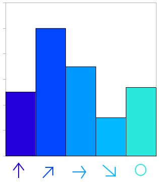
This post follow the same idea as Lots of features from color histograms on a directory of images but using Edge orientation histograms in global and local features.
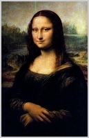
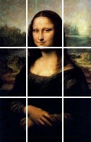
Basically I wanted to construct a collection of different edge orientation histograms for a collection of images that were saved in a directory. The histograms were calculated in different regions so I could get a lot of features. The images were numerated so the name of the file coincides with a number. The first thing I noticed was that I shouldn't use the code of Edge orientation histograms in global and local features directly because it was very inefficient. There is no need of calculating the gradients each time. It is better to do it just once and then extract the histogram from regions of this initial process. For this reason I divided that function in two functions: extract_edges and hist_edges. Here are both codes:
# parameters
# - the image
function [data] = extract_edges(im)
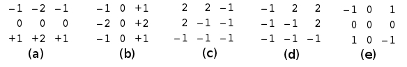
% define the filters for the 5 types of edges
f2 = zeros(3,3,5);
f2(:,:,1) = [1 2 1;0 0 0;-1 -2 -1];
f2(:,:,2) = [-1 0 1;-2 0 2;-1 0 1];
f2(:,:,3) = [2 2 -1;2 -1 -1; -1 -1 -1];
f2(:,:,4) = [-1 2 2; -1 -1 2; -1 -1 -1];
f2(:,:,5) = [-1 0 1;0 0 0;1 0 -1];
% the size of the image
ys = size(im,1);
xs = size(im,2);
# The image has to be in gray scale (intensities)
if (isrgb(im))
im = rgb2gray(im);
endif
# Build a new matrix of the same size of the image
# and 5 dimensions to save the gradients
im2 = zeros(ys,xs,5);
# iterate over the posible directions
for i = 1:5
# apply the sobel mask
im2(:,:,i) = filter2(f2(:,:,i), im);
end
# calculate the max sobel gradient
[mmax, maxp] = max(im2,[],3);
# save just the index (type) of the orientation
# and ignore the value of the gradient
im2 = maxp;
# detect the edges using the default Octave parameters
ime = edge(im, 'canny');
# multiply against the types of orientations detected
# by the Sobel masks
data = im2.*ime;
function [data] = histo_edges(im, edges, r)

% size of the image
ys = size(im,1);
xs = size(im,2);
size = round(ys/r) * round(xs/r);

# produce a structur to save all the bins of the
# histogram of each region
eoh = zeros(r,r,6);
# for each region
for j = 1:r
    for i = 1:r
        # extract the subimage
        clip = edges(round((j-1)*ys/r+1):round(j*ys/r),round((i-1)*xs/r+1):round(i*xs/r));
        # calculate the histogram for the region
        eoh(j,i,:) = (hist(makelinear(clip), 0:5)*100)/numel(clip);
    end
end

# take out the zeros
eoh = eoh(:,:,2:6);

# represent all the histograms on one vector
data = zeros(1,numel(eoh));
data(:) = eoh(:);
Now, with this two functions and following the idea of Lots of features from color histograms on a directory of images, it is possible to generate the features in just one vector for each of the images:
function [t_set] = extract_eohs(dir, samples, filename)

fibs = [1,2,3,5,8,13];
total = 0;
ranges = [6, 2];
for fib = 1:size(fibs)(2)
    ranges(fib,1) = total + 1;
    total += 5*fibs(fib)*fibs(fib);
    ranges(fib,2) = total;
endfor

histo = zeros(samples, total);

for ind = 1:samples
    im = imread(strcat(dir, int2str(ind)));
    edges = extract_edges(im);
    for fib = 1:size(fibs)(2)
        histo(ind,ranges(fib,1):ranges(fib,2)) = histo_edges(im, edges, fibs(fib));
    endfor
endfor
save("-text", filename, "histo");
save("-text", "ranges.dat", "ranges");

t_set = ranges;