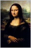
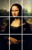
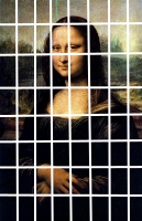
In a previous post I explained how to produce color or intensities histogram of different regions of an image. For example Fig 1, Fig 2 and Fig 3 presents the regions for three different type of region divisions: 1, 3, 8 respectively.

The basic goal was to produce small subimages of aproximately the same size and then calculate the histogram over the subimage. In this post I will use the existent function regionImHistogram  to produce features for a set of images that are in the same directory. The images are numerated in the directory to simplify the process and to track it back to the data I have in other tables

For each image I am going to produce a lot of features. The basic idea is to produce histograms of many regions. Concerned of the size of the descriptor I am going to stop using 256 bins for the histograms. Instead of that I am going to use different quantities of bins depending on the regions I am dividing the image. If I have more regions, I will use less bins. More regions also means less pixels, so maybe this will give a little bit more of generalization or statistical power to the feature. Here is the code for 6 different region divisions.

% Parameters:
% - directory with the images
% - number of images on the directory
% - name of the file with the features
function extract_cohs(dir, samples, filename)

% The different amount of regions the image
% is going to be divided
fibs = [1,2,3,5,8,13];
% The bins per region
bins = [128, 64, 32, 16, 8, 4];

% A counter of the number of features added
total = 0;
% The ranges that indicate were the set of features
% per region division are going to be saved
ranges = [6, 2];

% This cycle calculates the ranges in the vector
for fib = 1:size(fibs)(2)
    ranges(fib,1) = total + 1;
    total += 3*fibs(fib)*fibs(fib)*bins(fib);
    ranges(fib,2) = total;
endfor

% create the vector that is going to keep all the samples
histo = zeros(samples, total);

% open each image and process it
for ind = 1:samples
    im = imread(strcat(dir, int2str(ind)));
    for fib = 1:size(fibs)(2)
        histo(ind,ranges(fib,1):ranges(fib,2)) = regionImHistogram(im, fibs(fib), bins(fib));
    endfor
endfor

% save the features
save("-text", filename, "histo");

% save the values of the ranges
save("-text", "ranges.dat", "ranges");

The previous code will generate 6780 features per image and depending on the quantity of images it could take a while. It's quite straight forward to calculate intensity histograms from this code. Two changes are necessary:

1. Instead of

    total += 3*fibs(fib)*fibs(fib)*bins(fib);

You have to take out the 3*

    total += fibs(fib)*fibs(fib)*bins(fib);

2. After

    im = imread(strcat(dir, int2str(ind)));

You have to transform the image to grayscale

    im = imread(strcat(dir, int2str(ind)));
    if isrgb(im)
        im = rgb2gray(im)
    else

I ll be posting some code to produce edge orientation histogram very soon.