This is the last type of histograms I used in my project of training an Adaboost classifier to distinguish two artistic styles.

The basic idea in this step is to build a histogram with the directions of the gradients of the edges (borders or contours). It is possible to detect edges in an image but it in this we are interest in the detection of the angles. This is possible trough Sobel operators. The next five operators could give an idea of the strength of the gradient in five particular directions (Fig 1.).

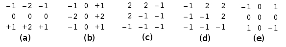
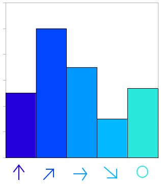
The convolution against each of this mask produce a matrix of the same size of the original image indicating the gradient (strength) of the edge in any particular direction. It is possible to count the max gradient in the final 5 matrix and use that to complete a histogram (Fig 2.)

In terms of avoiding the amount of non important gradients that could potentially be introduced by this methodology, an option is to just take into account the edges detected by a very robust method as the canny edge detector. This detector returns a matrix of the same size of the image with a 1 if there is an edge and 0 if there is not and edge. Basically it returns the contours of the objects inside the image. If you just consider the 1's we are just counting the most pronounced gradients.

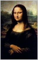
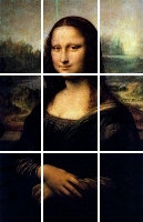
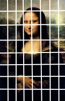
I am also interested in calculate global and local histograms (I have already talk about this in previous posts).  For example Fig 1, Fig 2 and Fig 3 presents the regions for three different type of region divisions: 1, 3, 8 respectively.

I found this code but I had to do several modifications because of my particular requirements. The most importants are:

• I need to work just with gray scale images
• I took out an initial filter that seems to be unnecessary
• I need to extract histograms of different regions
• I need a linear response. Just a vector with the responses together

I am posting the code with all the modifications:

# parameters
# - the image
# - the number of vertical and horizontal divisions
function [data] = edgeOrientationHistogram(im, r)

% define the filters for the 5 types of edges
f2 = zeros(3,3,5);
f2(:,:,1) = [1 2 1;0 0 0;-1 -2 -1];
f2(:,:,2) = [-1 0 1;-2 0 2;-1 0 1];
f2(:,:,3) = [2 2 -1;2 -1 -1; -1 -1 -1];
f2(:,:,4) = [-1 2 2; -1 -1 2; -1 -1 -1];
f2(:,:,5) = [-1 0 1;0 0 0;1 0 -1];

% the size of the image
ys = size(im,1);
xs = size(im,2);

# The image has to be in gray scale (intensities)
if (isrgb(im))
    im = rgb2gray(im);
endif

# Build a new matrix of the same size of the image
# and 5 dimensions to save the gradients
im2 = zeros(ys,xs,5);

# iterate over the posible directions
for i = 1:5
    # apply the sobel mask
    im2(:,:,i) = filter2(f2(:,:,i), im);
end

# calculate the max sobel gradient
[mmax, maxp] = max(im2,[],3);
# save just the index (type) of the orientation
# and ignore the value of the gradient
im2 = maxp;

# detect the edges using the default Octave parameters
ime = edge(im, 'canny');

# multiply against the types of orientations detected
# by the Sobel masks
im2 = im2.*ime;

# produce a structur to save all the bins of the
# histogram of each region
eoh = zeros(r,r,6);
# for each region
for j = 1:r
    for i = 1:r
        # extract the subimage
        clip = im2(round((j-1)*ys/r+1):round(j*ys/r),round((i-1)*xs/r+1):round(i*xs/r));
        # calculate the histogram for the region
        eoh(j,i,:) = (hist(makelinear(clip), 0:5)*100)/numel(clip);
    end
end

# take out the zeros
eoh = eoh(:,:,2:6);

# represent all the histograms on one vector
data = zeros(1,numel(eoh));
data(:) = eoh(:);

 
The makelinear function doesn't exist in Octave. All it does is converting a matrix into a vector. If the function doesn't exist you can use the following function.

# makelinear.m
# converts any input matrix into a 1D vector (output)

function data = makelinear(im)
data = zeros(numel(im),1);
data(:) = im(:);

In a previous post I explained how to produce color or intensities histogram of different regions of an image. For example Fig 1, Fig 2 and Fig 3 presents the regions for three different type of region divisions: 1, 3, 8 respectively.

The basic goal was to produce small subimages of aproximately the same size and then calculate the histogram over the subimage. In this post I will use the existent function regionImHistogram  to produce features for a set of images that are in the same directory. The images are numerated in the directory to simplify the process and to track it back to the data I have in other tables

For each image I am going to produce a lot of features. The basic idea is to produce histograms of many regions. Concerned of the size of the descriptor I am going to stop using 256 bins for the histograms. Instead of that I am going to use different quantities of bins depending on the regions I am dividing the image. If I have more regions, I will use less bins. More regions also means less pixels, so maybe this will give a little bit more of generalization or statistical power to the feature. Here is the code for 6 different region divisions.

% Parameters:
% - directory with the images
% - number of images on the directory
% - name of the file with the features
function extract_cohs(dir, samples, filename)

% The different amount of regions the image
% is going to be divided
fibs = [1,2,3,5,8,13];
% The bins per region
bins = [128, 64, 32, 16, 8, 4];

% A counter of the number of features added
total = 0;
% The ranges that indicate were the set of features
% per region division are going to be saved
ranges = [6, 2];

% This cycle calculates the ranges in the vector
for fib = 1:size(fibs)(2)
    ranges(fib,1) = total + 1;
    total += 3*fibs(fib)*fibs(fib)*bins(fib);
    ranges(fib,2) = total;
endfor

% create the vector that is going to keep all the samples
histo = zeros(samples, total);

% open each image and process it
for ind = 1:samples
    im = imread(strcat(dir, int2str(ind)));
    for fib = 1:size(fibs)(2)
        histo(ind,ranges(fib,1):ranges(fib,2)) = regionImHistogram(im, fibs(fib), bins(fib));
    endfor
endfor

% save the features
save("-text", filename, "histo");

% save the values of the ranges
save("-text", "ranges.dat", "ranges");

The previous code will generate 6780 features per image and depending on the quantity of images it could take a while. It's quite straight forward to calculate intensity histograms from this code. Two changes are necessary:

1. Instead of

    total += 3*fibs(fib)*fibs(fib)*bins(fib);

You have to take out the 3*

    total += fibs(fib)*fibs(fib)*bins(fib);

2. After

    im = imread(strcat(dir, int2str(ind)));

You have to transform the image to grayscale

    im = imread(strcat(dir, int2str(ind)));
    if isrgb(im)
        im = rgb2gray(im)
    else

I ll be posting some code to produce edge orientation histogram very soon.

In a previous post I explained how to produce color or intensities histogram of an image. In this post I will post some codes to produce them in different regions. The idea remains the same, however we are going to divide the image in different regions to obtain global and local histograms of the same image.

For example Fig 1, Fig 2 and Fig 3 presents the regions for three different type of region divisions: 1, 3, 8 respectively.

The basic goal is to produce small subimages of aproximately the same size and then calculate the histogram over the subimage. Here is the code.

function [data] = regionImHistogram(im, r, bins)

% 1. extract the x and y size of the image
ys = size(im,1);
xs = size(im,2);

% 2. calculate the number of pixels of each region
size = round(ys/r)*round(xs/r)

% 3. create a structure to keep all the histograms
coh = zeros(bins*3, r*r);

% 4. iterate over all the regions
for j = 1:r
    for i = 1:r
        %5. extract the subimage
        % 14/12/2016: this doesn't work - for some reason transform the crop two grayscale
        % clip = im(round((j-1)*ys/r+1):round(j*ys/r),round((i-1)*xs/r+1):round(i*xs/r));

        % 14/12/2016: Use this instead
        clip = imcrop(im,[round((i-1)*xs/r+1) round((j-1)*ys/r+1) round(xs/r)-1  round(ys/r)-1]);

        %6. calculate the histogram and normalize it
        coh(:,(j-1)*r+i) = linearHistogram(clip, bins)/size;
    end
end

% 7. put it all in just one vector
data = zeros(1,numel(coh));
data(:) = coh(:);

Notice that instruction 3 creates a matrix bins*3 x r*r. Remember that the color histograms has a histogram per color so it's three times the number of bins. And we are going to need one per block (3*3). Instruction 5. extract the subimage. Instruction 6. use the function explained in my previous post to build the color/intensity histogram. Instruction 7. is particularly important because I am generating descriptors for training my Adaboost classifier.

Then, this would be the code to produce the histograms of a 3x3 region division

% open the image
im = imread(path/to/image);
% call the function
linear = regionImHistogram(im, 3, 256);

Note that it is almost the same code to produce an intensity histograms of a 3x3 region division

% open the image
im = imread(path/to/image);
% transform to gray scale
im = im = rgb2gray(im);
% call the function
linear = regionImHistogram(im, 3, 256);

There is going to be a final post of how to use the regionImHistogram to generate multiple histograms of different regions and different amount of bins.

The bins of the color or intensities histograms are common features that are used in many kinds of applications. In my case, I am interested on them because I want them as the input of a classifier of images (Adaboost that I explained in my previous post). For that reason I have a couple extra requirements that I will explain later on this post.

There are different ways of representing the colors of an image. A very common and natural one is the combination of the three primary colors: Red, Green and Blue. Each pixel in an image is basically a combination of values of these three colors. The higher the value, the higher the intensity. These values are always in the range of 0 to 255. Then it is possible to think in a histogram of, for example, red for a particular image. We could have at most 256 bins (potentially less if we want to join several bins into one). Each bin would have the total number of pixels that have a particular intensity of red. Then, we repeat the process for green and blue.

I found this code that is able to build three histograms, one for each color by simple call:

% 1. Read the image
im = imread('/path/to/image');
% 2. Calculate the histogram with 256 bins
hist = imHistogram(im,256);

Moreover, you also can calculate intensities histograms by just transforming the color image into a gray scale image.  The main difference is that instead of three histograms for three colors the method is going to return just one histogram of 256 values with the intensities.

 
% 1. Read the image
im = imread('/path/to/image');
% 2. verify that it is a color image
if isrgb(im)
% 3. transform it
im = rgb2gray(im);
endif
% 4. calculate the histogram with 256 bins
hist = imHistogram(im,256);

This worked perfect on Octave (a free open source alternative to Matlab) but I had two small issues related with my particular problem:

1. I needed a linear representation of the histograms because I wanted to use the values as the input of a classifier (Adaboost that I explained in my previous post).  Instead of three separated histograms represented in different vectors of 256 bin each, I needed just one big vector of 768 with the three histograms next to the other. That was not difficult to solve.

 
% 1. read the image
im = imread('path/to/image');
% 2. calculate the histogram with 256 bins
hist = imHistogram(im,256);
% 3. make the vector of the right size (768)
linear = zeros(1,numel(hist));
% 4. copy the values to the new vector
linear(:) = hist(:);

2. My second problem was a bit more particular. I needed to process a big collection of images and I found out some of them were in gray scale. This cause an inconsistency in the size of the vectors. As I said before, the gray scale just have one value that defines the intensity instead of three values of the three colors. I solved it by copying the vector three times when I found that a image was gray (i.e. the imHistogram returns a vector of 256).

 
% 1. read the image
im = imread('/path/to/image');
% 2. check if it is gray
if !isrgb(im)
% 3. calculate the histogram with 256 bins
hist = imHistogram(im, 256);
% 4. create a new vector of the right size
linear = zeros(1,numel(hist));
% 5. copy the values to the new vector
linear(:) = hist(:);
endif

My final method looks like this:

%linearHistogram.m
function linear = linearHistogram(im, bins)
% check if it is a color image
if isrgb(im)
% calculate the histogram with 256 bins per color
hist = imHistogram(im, bins);
% create a new vector of the right size
linear = zeros(1,numel(hist));
% copy the values to the new vector
linear(:) = hist(:);
else
% calculate the histogram
hist = imHistogram(im, bins);
% create a new vector of three times the size
linear = zeros(1,length(hist)*3);
% set the same histogram to the three sections
linear(1:256) = linear(257:512) = linear(513:768) = hist(:);
endif

You can see that it receives the image as a parameter, so you need 2 instructions to call it.

 
% 1. Read the image
im = imread('/path/to/image');
% 2. Calculate the linear histogram with 256 bins
hist = linearHistogram(im,256);